User guide#
The main objective of orthoseg is to make it accessible to automatically digitize features on orthophotos. This manual will guide you through the process of setting up a new project, creating a training dataset, training a neural network and running a prediction on an orthophoto.
Run sample project#
Once the installation of orthoseg and its dependencies is completed, you can run the sample project included. The sample project is an easy way to get started and should give a good idea on how you can start your own segmentation project.
It contains:
a training dataset that can be used to train a network to detect football fields
a sample of the basic configuration for a typical project
a sample of the default directory structure used by orthoseg
a QGIS project file with the training data + aerial images that will be used to train the neural network + to detect football fields on
Remark: the training data included is meant to show how the process works, not to give perfect, or even decent, results.
Running the sample project is easy. If the installation was successful, the following steps should do the trick:
start a conda command prompt
activate the orthoseg environment with:
conda activate orthoseg
download the sample projects from orthoseg. You can specify the base location to download the sample projects to, but in this tutorial I’ll assume “~” (= your home directory) for simplicity:
orthoseg_load_sampleprojects ~
preload the images so they are ready to detect the football fields on, using the sample configurations file “footballfields.ini_BEFL-2019”:
orthoseg_load_images --config ~/orthoseg/sample_projects/footballfields/footballfields_BEFL-2019.ini
for the footballfields sample project, a pretrained neural network was downloaded in step orthoseg_load_sampleprojects to avoid having to train it. But, normally you would now train the neural network with the following command:
orthoseg_train --config ~/orthoseg/sample_projects/footballfields/footballfields.ini
detect the football fields:
orthoseg_predict --config ~/orthoseg/sample_projects/footballfields/footballfields_BEFL-2019.ini
Now, the directory ~/orthoseg/sample_projects/footballfields/output_vector will contain a .gpkg file with the football fields found.
An interesting exercise might be to detect football fields on another layer (on another location). To get reasonable results, this should be a layer with 0.25 meter pixel size, as this was the pixel size the footballfields detection was trained on. It’s best to first read Prepare a new project for some background information and then you could try the following steps:
add the layer you want to predict on to the imagelayer.ini config file
make a copy of footballfields_BEFL-2019.ini and change the predict image_layer parameter in the file to point to the new layer:
[predict]
image_layer = BEFL-2019
run orthoseg_load_images to prepare the layer to predict on:
orthoseg_load_images –config ~/orthoseg/sample_projects/footballfields/footballfields_BEFL-2019.ini
run the detection again with orthoseg_predict:
orthoseg_predict –config ~/orthoseg/sample_projects/footballfields/footballfields_BEFL-2019.ini
Prepare a new project#
A few technical steps need to be taken to prepare a new segmentation project.
1. Only once: prepare “projects” directory#
If this is your very first orthoseg project, you need to prepare a directory where you want to put your orthoseg projects. In the rest of the documentation we’ll refer to this directory as {projects_dir}.
It doesn’t really matter where this directory is located, but these are examples that can give you some inspiration:
on linux: ~/orthoseg/projects
on windows: c:/users/{username}/orthoseg/projects
The easiest way to create it is by starting from a copy of the sample_projects directory to eg. your personal orthoseg directory and rename it to projects.
This way your projects directory immediately contains:
an imagelayers.ini file (with sample content)
a project_defaults_overrule.ini file (with sample content)
the project_template directory: the template for a new segmentation project
2. Add the layer(s) you want to segment on to the image layer configuration#
The configuration for the image layers is located in {projects_dir}/imagelayers.ini.
Layers can be accessed from a WMS server, a WMTS server or via a file (= a GDAL raster dataset). The basic structure of this configuration file is as follows: every section in the .ini file (eg. [BEFL-2019]) contains the configuration of one image layer. In later steps of this tutorial you well need to use the “image layer names” (for these examples BEFL-2019 and BEFL-2020), they are referred to with {image_layer_name}:
# In this file, the image layers we can use in segmentations are configured.

[BEFL-2019]
# Configuration info of this layer
...

[BEFL-2020]
# Configuration info of this layer
...
A “file layer” can be any local file in one of the many raster file types supported by GDAL. Via the “file layer”, you can also use the GDAL WMS driver by creating an xml file with the necessary configuration. An example file to use a XYZ tile server (eg. OpenStreetMap) can be found here: imagelayer_osm.xml.
A more elaborate example that can be used as a template for the configuration can be found here: imagelayers.ini.
3. Project name#
Choose a new name for the segmentation project: par example ‘greenhouses’, ‘trees’, ‘buildings’,… In the rest of the manual the project name will be refered to with {segment_subject}.
4. Prepare “project” directory#
For your new segmentation project, make a copy of the project_template directory to {projects_dir} and rename it to {segment_subject}.
5. Prepare project settings#
Rename the project file in the new project directory from projectfile.ini to {segment_subject}.ini. In the file you should at least change the following parameter::
[general]
segment_subject = {segment_subject}
As you might have recognized from the small section above, orthoseg uses the good old .ini file format for its configuration, with “ExtendedInterpolation”. General information about this file format can be found here: ConfigParser-ExtendeInterpolation.
The configuration can be found + modified in the following files:
All existing sections and parameters + their default values can be found in the following file: orthoseg_install_dir/orthoseg/project_defaults.ini. It is highly recommended not to change anything in this file, as it will be overwritten when installing a new version of orthoseg anyway. But if you want to overrule any setting, this is the perfect spot to find all existing sections + parameters and copy/paste the section + parameter to one of the next files and change the value there to overrule it for your project(s).
If you want to overrule a parameter for all the projects in your project directory, add the section + parameter to the project_defaults_overrule.ini file in your projects directory, eg: {projects_dir}/project_defaults_overrule.ini.
If you want to overrule parameters for a specific project, you can do so in the project-specific config file: eg. {projects_dir}/{segment_subject}/{segment_subject}.ini.
6. Configure image layer(s)#
If the image layers you want to train/predict on aren’t configured yet, configure them in {projects_dir}/imagelayers.ini, the same way as the default layers provided.
7. Prepare training data files#
The labels folder in the new project folder contains two .gpkg files where training examples can be added to as explained in the following page of this manual. The file names should have the following structure:
{segment_subject}_{image_layer_name}_locations.gpkg
{segment_subject}_{image_layer_name}_polygons.gpkg
If you want to create one segmentation with training examples based on multiple image layers, you can create a seperate pair of .gpkg files per image layer.
8. Prepare GIS project#
Start your prefered GIS application (eg. QGIS), and create a new project. Add the .gpkg files from the labels directory and add the layers you want to digitize the training examples on (eg. BEFL-2019).
It is practical to create a layer group per image layer you want to train data on with:
the 2 corresponding .gpkg files
the image layer (eg. BEFL-2019)
Save the project to the project directory.
Create training data#
General info#
You can use any GIS tool you want to create the training data, as long as it can edit .gpkg files. I personally use QGIS on a windows computer, but even though in some cases I might give specific instructions based on the environment I use, I’m sure valid alternatives exist using any other GIS tool on eg. linux.
Before you start digitizing examples, it is a good idea to put a definition of the subject you want to segment on paper, with a clear scope of things you want to include or want to exclude. While you are busy creating your training dataset this might still evolve based on examples you encounter and didn’t think of at this stage, but as it is important that the training dataset is consequent, make sure the definition is/stays clear.
The orthoseg training data is (by default) organized as follows. In your {project_dir} there is a directory called labels. In this directory there should be 2 files per image layer that you want to use to base your training on:
{segment_subject}_{image_layer_name}_locations.gpkg
{segment_subject}_{image_layer_name}_polygons.gpkg
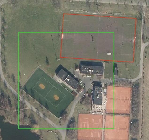
In the locations` file you need to draw the bounding boxes of the images that will be downloaded and used as the images to train the detection on. In the polygons` file you need to digitize the things you want to detect as polygons as shown in the screenshot below. The green square is the location, the red rectangle is the polygon drawn to show where the football field is in the location. This training example will help the neural network to learn how a (part of a) football field looks, but also that tennis fields are not to be detected…
Creating training data is -in my experience- an iterative process. You add some samples to the training dataset, you evaluate the results, add some more,… This way you can minimize the number of training samples you need to digitize/train on which can save a lot of time.
So, the following steps need to be iterated over till you are happy with the results:
Search for good examples and add them to the training input#
There are different strategies possible to find good examples to add to the training input:
1. On random locations#
For the initial examples, you can use an existing dataset to find relevant locations or just zoom to random locations distributed over the territory you want to segment.
2. Use the vectorized result of a prediction on the entire territory#
If a run has been done on the entire territory, a vectorized file of the segmentation will be available. Using this, there are several options to look for new examples using it:
Do overlays with existing datasets that can help to find missing examples.
Check locations in a random way distributed on the territory to find segmentation errors.
In the vector file of the segmentation result, a column “nbcoords” will be available. Order this column descending to find the polygons with the most points: often these polygons with many points are bad segmentations.
3. Use the result of a previous training run#
If you already did a training run, it is often useful to look for errors in the training data. After training, orthoseg will automatically run an “evaluation” prediction on all the images in the training, validation and test datasets. This won’t be saved as a vector file, but these predictions will be saved as images in the following directories:
{project_dir}/training/{traindata_version}/train/{segment_subject}_…_eval
{project_dir}/training/{traindata_version}/validation/{segment_subject}_…_eval
{project_dir}/training/{traindata_version}/test/{segment_subject}_…_eval
Each of these directories is useful to look at in the following way:
If you open the directory with the predictions and set the view in eg. “Windows explorer” to “large tiles”, you will see the original image, followed by the mask and by the prediction, so you can easily compare them.
The file names of the predictions are formatted this way: <prediction_quality>_<x_min>_<y_min>_<x_max>_<y_max>_<nb_pix_x>_<nb_pix_y>_<image_type>.tif
<prediction_quality>: is the percentage overlap between the mask (as digitized in the training dataset) and the prediction, so examples with problems will have a small percentage overlap and will be shown first in the directory.
<x_min>,…: these are the coordinates of the location of the image. So if you want to correct a digitization of an image in eg. QGIS, you can:
copy/paste the <x_min>_<y_min> to the “coordinate” field the status bar (below) in QGIS
replace the “_” by “,”
press the ENTER key, and you’ll be in the right location.
<image_type>: ‘mask’ for the digitized mask, ‘pred’ for the prediction,…
4. Add good examples found to the training dataset#
The way you digitize the examples in the training dataset will influence the quality of the result significantly, so here is some advice:
Digitize the examples for the training process as precise as you want the result to be.
If you need relatively complex interpretation yourself to deduct things from the image, the AI probably won’t succeed in doing it… yet. An example of something I didn’t get good results with:
A road that goes into a forest and comes out of it a bit further might be logic to a human that it will probably continue under the trees, but this didn’t work in my quick tests.
If you want detailed results, make sure you digitize the examples on the same ortho imagery you are going to train the network on. Certainly for subjects that have a certain height (eg. buildings, trees,…) a significant translation of eg. the roof can occur between different acquisitions that can influence the accuracy.
With the default parameters, the training works on images of 512x512 pixels and the prediction on 2304x2304. So the AI won’t be able to take into account more information than available on those images. So if you need to zoom out and look on larger area’s than those, take in account the AI won’t have this option.
If you find good examples, you can add them to the training dataset as such:
First, add the location that will be used to determine the extent of the image to the {subject}_{image_layer_name}_locations file. The bounding box of the image generated for the training process will be the minx and miny of the bounding box of the polygon digitized. The width and height of the image are determined by the pixel width and pixel height as defined in the configuration files. Par example, using the default pixel width and height of 512 pixels, and a pixel size of 0.25 meter/pixel the image width and height will be 128 meter (512 pixels * 0.25 meter/pixel). The location polygon should be digitized at least the size the generated image will be, so it is clear for which area you need to digitize the exact labeled polygons in the next step. During the training step the locations will be validated and if (some of them) are too small, an error will be given. The Advanced digitizing panel in QGIS makes it quite trivial to digitize them with the correct size.
You need to fill out the following properties for each location:
traindata_type (text): determines how the image generated based on this location will be used in the training. Possible values: ‘train’, ‘validation’, ‘test’, ‘todo’.
locations set to ‘train’ will actually be used to train the AI on.
locations set to ‘validation’ will be used during the training to crosscheck if the AI is sufficiently learning in a general way so it will be working well on data it has never seen before instead of specializing on the specific cases in the ‘train’ locations. The best results are obtained if 10% to 20% of the locations are set to ‘validation’ and try to focus on as many different common examples as possible, but evade including difficult situations in the ‘validation’, only set those to ‘train’.
optionally, you can set locations to ‘test’: they won’t be used in the training process, but after the training run the segmentation will be applied to them, including reporting. Eg. if you have an existing dataset with examples of moderate quality or if you encounter situations you are not sure about, you can set them to ‘test’.
optionally, you can set locations to ‘todo’: they won’t be used at all, but this class is practical to signify that the location still needs work: eg. the polygons still need to be digitized.
description (text): optional: a description of the label location
Remark:
train images can’t/won’t overlap: when looping through the locations digitized, if an image location overlaps with an already generated image, it will be skipped.
If you are adding a ‘false positive’, so a location where the segmentation thinks the subject is present on this location, but it isn’t, you are already ready and can look for another example.
If you are adding a ‘false negative’, or any new example, now you need to digitize the actual subject in the {subject}_labeldata file. It is important to digitize all samples of the subject in the location area added in the previous step, as any surface that isn’t digitized will be treated (and trained) as a ‘false positive’.
The following properties need to be filled out:
label_name (text): the content of the label data digitized. The label names you can use are defined in the subjects configuration file. If it is different than the ones specified there, it will be ignored.
description (text): optional: a description of the feature digitized.
Run training + (optionally) a (full) prediction#
Instructions to run a train, predict,… session can be found in the next section.
Run train, predict,… session#
Once you have added a meaningful number of (extra) examples, you can do a (new) training run. The number of added examples that is meaningful will depend on the case, but a reasonable amount is 50. Once the model is trained, you can continue by running a prediction and if wanted a postprocessing step.
If you ran the sample project, these steps will look very familiar:
start a conda command prompt
activate the orthoseg environment with:
conda activate orthoseg
preload the images so they are ready to detect your {segment_subject} on, using the configuration file {project_dir}{segment_subject}.ini:
orthoseg_load_images –config {project_dir}{segment_subject}.ini
train a neural network to detect football fields:
orthoseg_train –config {project_dir}{segment_subject}.ini
detect the football fields:
orthoseg_predict –config {project_dir}{segment_subject}.ini
After this completes, the directory {project_dir}/output_vector will contain a .gpkg file with the features found.
Of course it is also possible to script this in your scripting language of choice to automate this further…
Remark:#
Because tasks often take quite a while, orthoseg maximally tries to resume work that was started but was not finished yet. Eg. when predicting a large area, OrthoSeg will save the prediction per image, so if the prediction process is stopped for any reason and restarted, it will continue where it stopped.